Matrix-vector multiplication methods |
Revision: 7/8/12
``Specializers'' are ways of constructing a multiplier for a particular matrix M, given M. In some cases, these specializers do not really specialize at all: they are just generic methods that are applied to M (the standard, naive implementation of the S-m-n theorem). In other cases, they depend critically on M, incorporating values from M directly into the generated code. Other cases fall somewhere in the middle: these specializers use methods that might be considered generic, but would be awkward because of the many cases the generic version would have to deal with. Note that, in most cases, whether generating specialized code or using generic code, the data itself has to be reorganized. That is, when we say a method is ``generic,'' we mean simply that it does not require the generation of new code at run time; it may still involve some latency in the form of data restructuring.
``Splitters'' are ways of partitioning matrices so that different
specializers can be applied to different parts.
With a few exceptions, specializers can be applied to any
matrix, so that if we partition a matrix into two parts, we can
apply arbitrary specializers to each parts.
Each value of M is handled by just one specializer,
and each is coded to add to each value of the output
vector w (that is, all assignments to w have the form
w[i] += ...), so in principle, we can do the multiplications
for the various partitions in any order.
There are exceptions, where a specializer can be applied only after
a particular splitter has been applied, and then that specializer
can be used only for the first of the partitions;
for example, OSKI can be used only after the matrix has been split
into one portion whose size is an exact multiple of the block size
(handled by OSK), and the remaining elements (a small number of
elements from the right side and bottom of the matrix).
In this note, we explain the various methods. We assuming we are multiplying matrix M by input vector v>, and producing output vector w. We only handle square matrices, of size n x n; the number of non-zeros is nz. We sometimes refer to the matrix as a set of triples <r, c, v>, giving the location and value of each non-zero (where we assume indexing from zero). This is not the representation actually used in any of our codes, but is the simplest one. (The generators described in WP 4 all start with this representation, where the elements are given in row-major order.)
This WP describes the algorithms in some detail. For a discussion of low-level coding details, see WP 3.
Specializers
In these descriptions, we mostly just describe how each method works. Occasionally, we discuss performance issues. There are several issues that come up:
- Instruction count is the most obvious consideration. It is usually fairly easy to see how the methods differ here, although it can depend on how well compilers perform various optimizations, which is non-obvious (and can differ among compilers).
- Memory behavior needs to be considered relative to the input and output vectors. In all cases, the matrix values themselves are laid out in memory so as to be consumed sequentially; no improvement is possible. However, accesses to v and w can be random, which would produce poor performance, or with a high degree of locality.
- Zero fill refers to the addition of zero values to the representation of M, which is required by some methods. In these cases, the amount of fill will very from matrix to matrix, and will be a crucial determinant of the method's performance.
- Vectorizability is the amenability of some methods to vectorization, which is a matter of being able to so arrange the data that large segments of contiguous elements of M can be simultaneously multiplied by contiguous elements of v. Most of our codes are not vectorizable, and those that are require some zero fill, which, as just noted, is going to mitigate the advantage of vectorizing.
Unfolding
The simplest method is to create a straight-line program that does all the floating-point operations. If the matrix elements are <r, c, v>, <r', c', v'>, ..., we could generate code
w[r] += v[c] * v;
w[r'] += v[c'] * v';
and so on. If r=r', it turns out to be somewhat more efficient to write this as:
w[r] = v[c] * v
 + v[c'] * v' + ...;
with exactly one assignment statement per row.
If M is very strongly banded - i.e. has few out-of-band elements - then the memory behavior will be very good. But if not, this approach can produce sub-optimal memory behavior relative to the input vector, in that it runs through large parts of v for each assignment. The method can be blocked. It has integer parameters b_r and b_c giving the block parameters. The matrix is conceptually divided into blocks of size b_r x b_c and computations are done on entire blocks (with the blocks themselves ordered in row-major order). The effect is to have more assignment statements - at most, n x b_c - which tends to lead to higher instruction counts. (If b_c = n, we will produce the code given above, with exactly n assignment statements; in practice, we have always found this to be more efficient.)
Unrolling
The standard compressed-sparse-row (CSR) data layout consists of three arrays:
- values is an array of floating-point numbers (doubles, in our experiments) of length nz, containing the non-zero elements of M in row-major order
- cols is an integer array of length nz giving the columns containing non-zeros in the first row, followed by the columns containing non-zeros in the second row, etc.
- rows is an integer array of length nz+1, which gives, in a somewhat convoluted way, the number of non-zeros in each row. It can be described this way: row[0] = 0, and for all i, row[i+1]-row[i] is the number of non-zeros in row i of M. Another way of looking at it is that row[i] is the location in values where the values in row i begin.
    for (i = 0; i<n; i++) {
       ww = 0.0;
       k = rows[i];
       kk = rows[i+1];
       for (; k <= kk-1; k += 1) {
          ww += mvalues[k]*v[cols[k]];
       }
       w[i] += ww;
     }
The unrolling specializer is this code, with partial unrolling of the inner loop (the unrolling factor being given by a parameter). See WP 3 for an example.
OSKI
Our version of OSKI is the ``register-blocking'' code described in Berkeley paper on OSKI. The idea is to block the matrix in small blocks (say, 2 x 2). Now consider the set of all non-zero blocks, meaning blocks that have at least one non-zero. Write a single, efficient loop that handles all blocks. For example, here is a loop for a 2 x 2 block:
to be filled in
The idea is that very efficient code can be generated for this loop. (In fact, it could even be vectorized, although it certainly would not be worthwhile because it does not have enough iterations to overcome the overhead of using vector instructions.) However, it introduces multiplications by zero, so increases the overall floating-point instruction count; this ``fill factor'' substantially determines whether this method will be efficient. In our experience, 1x2, 2x1, and 2x2 blocks are occasionally efficient, but larger blocks never are; obviously, this depends entirely on the matrix.
CSRbyNZ
Like unrolling and OSKI, the idea of CSRbyNZ is to produce loops with longer straight-line bodies, allowing for efficienct code (i.e. efficient register and pipeline usage). Here, we partition the rows of the matrix according to the number of non-zero elements, and generate a loop for each non-zero count.
For example, here is one loop from the CSRbyNZ code for matrix fidap005:
  for (i=0; i<6; i++) {
    row = rows1[a1];
    a1++;
    w[row] += mvalues1[b1+0] * v[cols1[b1+0]] + mvalues1[b1+1] * v[cols1[b1+1]]
            + mvalues1[b1+2] * v[cols1[b1+2]] + mvalues1[b1+3] * v[cols1[b1+3]]
            + mvalues1[b1+4] * v[cols1[b1+4]] + mvalues1[b1+5] * v[cols1[b1+5]]
            + mvalues1[b1+6] * v[cols1[b1+6]] + mvalues1[b1+7] * v[cols1[b1+7]]
            + mvalues1[b1+8] * v[cols1[b1+8]] + mvalues1[b1+9] * v[cols1[b1+9]]
            + mvalues1[b1+10] * v[cols1[b1+10]] + mvalues1[b1+11] * v[cols1[b1+11]];
      b1 += 12;
   }
For this matrix, there are exactly six rows that have 12 non-zeros, and this loop handles just those six rows. (This small matrix has exactly four loops; every row has either 6, 9, 12, or 15 non-zeroes. Most matrices have a greater variety of non-zero counts.) The mvalues1 array contains the non-zeros of m in just the order in which they are consumed by these loops (with b1 giving the current index into it).
This loop is not vectorizable because it accesses the input vector indirectly through the cols array (like unrolling). Still, it tends to be quite efficient because the long loop bodies are compiled efficiently and the overall code size is modest (since there are usually not too many distinct non-zero counts and therefore not too many loops).
Stencil
Where CSRbyNZ divides up the rows of M according to the number of non-zeros, stencil divides them up according to the exact pattern of non-zeros. Specifically, the stencil of each row is the location of the non-zeroes relative to the diagonal. E.g., if row r has non-zeroes in columns r-1, r, r+1, and r-3, its stencil would be {-1, 0, 1, 3}.
After dividing the matrix according to stencils, a separate loop is created for each stencil, which handles all the rows that have that stencil. For example, fidap005 has exactly three rows - rows 2, 4, and 6 - whose stencil is {-1, 0, 1, 8, 9, 10, 17, 18, 19}. These three rows are handled by this loop:
   int stencil1_2[3] = {2, 4, 6};
   for (i=0; i<3; i++) {
      row = stencil1_2[i];
      vv = v+row;
      w[row] += vv[-1] * mvals1[0] + vv[0] * mvals1[1]
              + vv[1] * mvals1[2] + vv[8] * mvals1[3]
              + vv[9] * mvals1[4] + vv[10] * mvals1[5]
              + vv[17] * mvals1[6] + vv[18] * mvals1[7]
              + vv[19] * mvals1[8];
      mvals1 = mvals1 + 9;
   }
The values of M are laid out in the order in which they are consumed by these loops.
Stencil loops can be compiled to very efficient code, because they
do not have indirection through the cols array,
as in unrolling and CSRbyNZ.
Thus, we have found this to be the most efficient method for many matrices.
On the other hand, arrays can have many stencils, so
the code can get quite large, reducing its efficiency.
(The number of stencils in an array can be reduced in a variety
of ways, including simply swapping rows, and there is some
literature on this topic;
but this process is so combinatorially explosive that
we assume it could not be applied in real-time, so we have not
attempted to do it.)
We note also that stencil - and the same can be said of CSRbyNZ -
does not have particularly good memory behavior relative to either
the input or output vector, since each stencil loop may cover
rows that are randomly distributed throughout M
(and therefore affect randomly-distributed elements of w),
and each stencil contains elements randomly distributed throughout
a single row
(and therefore reads randomly-distributed elements of v).
One way of limiting the number of stencils - and, simultaneously, the cost of calculating the stencils - is to extract a band from M and apply stencil to that, handling the out-of-band elements by some other method. In previous work, we implemented this as a separate specializer, "banded stencil," but now we handle it by splitting the matrix into an in-band matrix and an out-of-band matrix, and using stencil for the first.
Row-segment
The idea of row-segment (and diagonal) is to allow for vectorization of the inner loop of the multiplication. Sparse matrices do not usually have non-zeros distributed consecutively; there are usually denser segments (e.g. around the diagonal) and less dense segments, but we do not generally see long segments of each row consisting entirely of nonzeros. Rather, the nonzeros tend to be distributed more randomly, and therefore accessed indirectly. This makes the inner loop difficult to vectorize.
To allow for vectorization, some non-zeros have to be included, creating additional overhead. Thus, these methods will be useful only if the portions of the matrix that are to be handled by vectorization are sufficiently dense. Representing all numbers by doubles means that, for most machines, the vectorization unit can achieve at best a two-fold speed-up; if the portion of M in question is less than 50% non-zeroes, vectorization cannot provide speed-up; due to overheads, it will probably slow the computation down in those cases. (The one previous method that does include zeroes is OSKI, where indeed the "fill factor" is a crucial determinant of the efficiency of the method. OSKI could in principle be vectorized, but because it rarely --- never, in our examples --- provides efficiency for block sizes greater than 2 x 2, vectorization would be pointless, as the speed-up would be overwhelmed by the overhead.)
Row-segment applies only to perfectly-banded matrices,
that is, matrices that have no non-zeroes outside of a defined
band around the diagonal
(although there may be some zeroes within the band).
Most matrices are not so strongly banded, so
in practice, this means it applies only to matrices
that result from using the
split_by_band or split_by_band2 splitter;
thus, this method requires that one of those be applied first.
One way to think of row-segment is that it pretends that every
row has a stencil consisting of consecutive indices
-lo, -lo+1, ..., -1, 0, 1, ..., hi.
Then for each row r, values M[r, r-lo], \ldots, M[r, r+hi]
are multiplied by v[r-lo], ..., v[r+hi], and the
result sum is added to w[r].
One question is how to deal with the first and last rows;
since M[0, -lo] and v[lo] do not exist, the description in
the previous paragraph is not complete.
In fact, we have two ways of dealing with this at the moment.
The method employed depends upon whether
split_by_band or split_by_band2 was used.
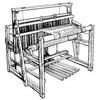
The two methods are illustrated here:
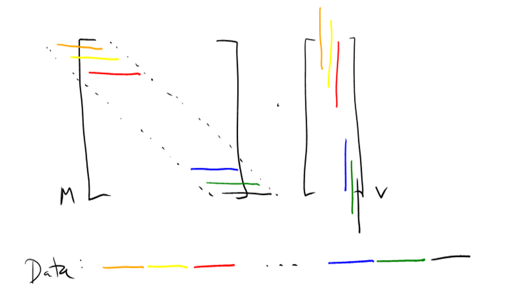
In each illustration, we are assuming a band of width 5 (lo=2 and hi=2). The band itself is shown as a dotted black line. The values of a particular color in M are multiplied by the elements of the same color in v. The illustration on the left shows row-segment used after split_by_band, and the one on the right shows it after split_by_band2, the difference being in how the first two and last two rows are handled. split_by_band includes all elements within the band. This means the first two and last two rows are short; we need to add two zeros to the first and last rows, and one zero to the second and second-to-last rows. More importantly, to avoid having a conditional in the main loop, v must be extended at the start and end, so that indices -2, -1, n, and n+1 are valid. This means that at the start of the multiplication, we need to allocate a vector of size n+4 and copy v into it, initializing the first two and last two elements to zero. To avoid this copying, split_by_band2 includes only elements within the band in rows that contain the entire band. This means excluding all elements in the first two and last two rows.
We believe that the copying required when using split_by_band will have only a small impact on the cost of the multiplication, but we believe that leaving off the first and last few rows (having them be handled by the secondary specializer) will have an even smaller impact. So we expect that experiments will show that using split_by_band2 will always be preferable, and then split_by_band (for this specializer) will be dropped. But that remains for the future.
Here is an example of row-segment applied to a (5, 5) band of fidap005 (n=27):
   mptr = mvalues1;
   for (r = 5; r < 22; r++) {
      ww = 0.0;
      v3 = v+r-5;
      for (i = 0; i < 11; i++) {
         ww += mptr[i] * v3[i];
      }
      w[r] += ww;
      mptr = mptr + 11;
   }
The inner loop should be easily vectorizable.
See the next section for a comparison of this method with diagonal.
Diagonal
This specializer is similar to row-segment in that it applies
only to the in-band portion of a matrix.
diagonal can be applied only after using
split_by_band or split_by_dense_band.
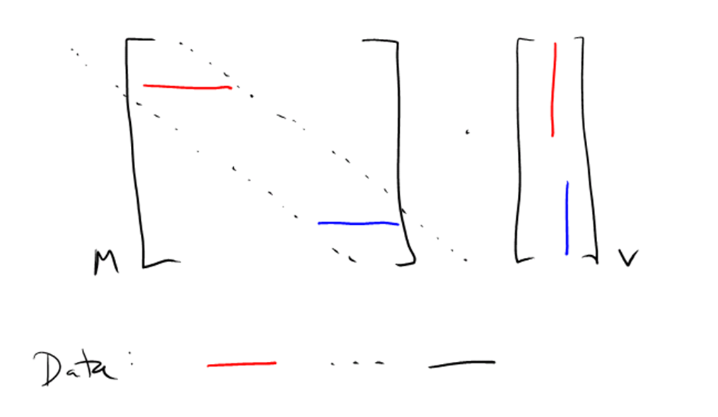
The idea is to store the values of each diagonal
consecutively, as shown in the figure below.
At each iteration, we handle one diagonal: multiply each value
of the diagonal by the corresponding value of v, and add it
to the corresponding value of w.
Here is the code generated for fidap005 with a (5, 5) band:
   m1 = mvalues1;
   for (i=0; i<11; i++) {
      diag = diags1[i];
      sz = 27-(diag<0 ? -diag :diag);
      fstrow = diag<0 ? -diag : 0;
      fstcol = diag<0 ? 0 : diag;
      w1 = w+fstrow;
      v1 = v+fstcol;
      for (j=0; j<sz; j++) {
         w1[j] += m1[j]*v1[j];
      }
      m1 += sz;
   }
The first several assignments are finding the size of the particular diagonal (a diagonal k columns to the left or right of the main diagonal has length n-k). The main loop is again a simple product of a diagonal from M with a large portion of v, and should be easily vectorizable.
row-segment vs. diagonal
row-segment and diagonal are both expected to be efficient only if they can take advantage of vectorization; otherwise, because their coding is not especially efficient and they introduce additional computation (zero calculations), they would probably not be competitive with other methods. Only experimentation will determine which is better in which cases, but here we provide some thoughts as to why each might be efficient in some circumstances. Note first that, broadly speaking, the number of zeros introduced by the two methods is the same --- it is just the number of zeros within the band. For this discussion, we define width as hi+lo+1.
-
row-segment will normally vectorize a much smaller
number of elements than diagonal --- namely
width vs. (approximately) n.
Therefore, more will be paid in overhead using row-segment.
- We may be able to more effectively reduce the fill factor
using diagonal by only including diagonals that are
sufficiently dense (which is the purpose of
split_by_dense_band).
In principle, we could do this with row segments as well, but
in practice row segments tend to all have more or less the same
density, while diagonals can vary greatly.
- row-segment has much better memory locality
than diagonal.
In fact, row-segment has pretty much optimal memory
behavior (it touches a small segment of v and exactly one
element of w on each iteration),
and diagonal has pretty much pessimal memory
behavior (it touches all of v and w on each iteration).
(It is possible to block diagonal; we have not
implemented that yet.)
- row-segment also has inherently better memory behavior, in that it touches each element of w just once, while diagonal touches each element of w width times.
Splitters
We will go into much less detail on splitters, because they are simpler and because we do not know that they will all be useful.
split-by-band, split-by-band2, and split-by-dense-band
These were discussed in the sections above on row-segment and diagonal. They all select elements from a band around the main diagonal. split-by-band2 is distinguished from the others in that it also cuts off the first and last few rows so as to ensure that only rows that contain a complete band are included; this simplifies the coding of row-stencil, but is not helpful for diagonal. split-by-dense-band is like split-by-band, but includes an additional parameter, giving the percentage of values in a diagonal that must be non-zero for that diagonal to be included in the partition. (A not-unreasonable strategy is to use split-by-dense-band with a very large band, and a third argument of, say, 80, ensuring that every diagonal that is at least 80% dense will be handled by a vectorizable loop.) Note that split-by-dense-band with a third argument of zero is equivalent to split-by-band (so split-by-band is really superfluous).
split-by-block
For specialization methods that use blocking, there may be a question of how to handle the "left-over" elements that do not belong to a full block; these occur in the columns at the far right and the bottom rows. In our case, the only method where this is an issue is OSKI. (Unfolding can use blocking as well, but there is no difficulty in handling partial blocks.) Rather than build in a method of handling these orphaned elements, we require that, to use OSKI, split-by-block must be used to extract all the complete blocks from M. If the blocks are of size b_r x b_c, let n_r be the largest multiple of b_r less than n, and let n_c be the largest multiple of b_c less than n. The first matrix returned by this splitter contains all elements <r, c, v> such that r < n_r and c < n_c.
split-by-stencil
A problem with using the stencil specializer is that a matrix may have very many stencils, and the resulting code can be inefficient just because of its size. One strategy is to generate stencil loops only for a limited number of stencils and use a different specializer for the remaining elements.
It is not clear what is the best way to select a subset of the stencils. This splitter uses a simple method: Its argument is an integer k. List the stencils of M in descending order of their coverage - the number of elements in rows that have this stencil, or the stencil's length times its popularity. Then selects enough stencils to cover no more than k elements. Note that this splitter always selects entire rows.
split-by-rownz
This splitter performs the same function for CSRbyNZ that split-by-stencil does for stencil - selecting only the row non-zero counts that have the greatest coverage, so as to avoid generating too many loops. In fact, as noted above, there are usually a small number of non-zero counts - much smaller than the number of stencils - so this splitter probably has little value.
Last updated on Fri Jul 6 09:00:35 CDT 2012